Skip to main content Skip to page footer

Mechanics of Materials

Topic: State of Stress

Here you will learn about how stress is defined in components and how it is conveniently divided into different components. Discover how to calculate the stresses that occur in a body when it is subjected to external forces, and how a known stress state is transformed into any arbitrary section plane. Learn how to determine the maximum stresses and in which section planes they act. Explore how to draw Mohr's circle and how to read the relevant information from it.

Let's explore these important concepts together.

3. Plane Stress State

Repetition in the Chapter Introduction

The plane stress state (also known as biaxial stress state or two-dimensional stress state) occurs when there is a two-dimensional load.

This happens in an element that is cut from a thin plate and is loaded only within its plane:
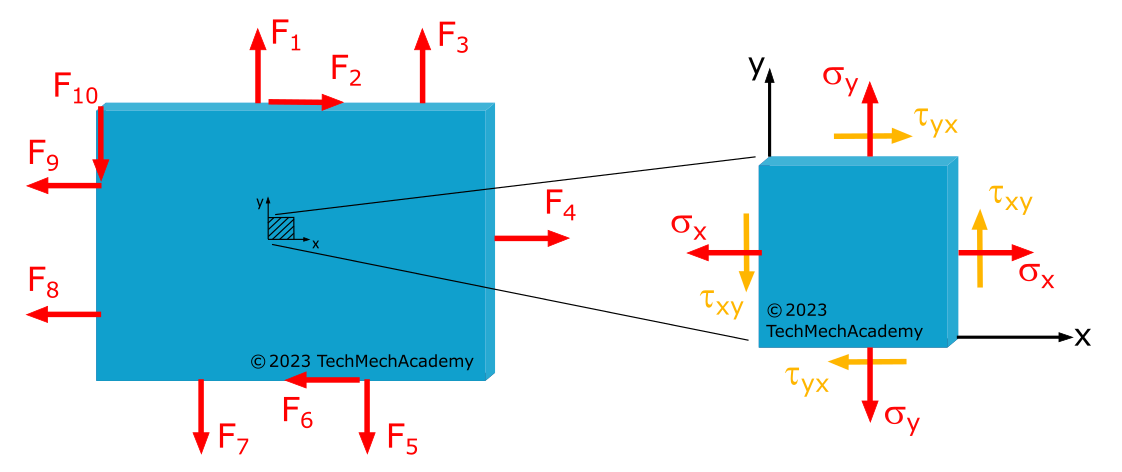
This figure shows the plane stress state.
Fig. 1.3.1: Plane Stress State for an x, y plane

Figure 1.3.1 shows a disc loaded in the \(x, y\)-plane, with no load in the \(z\)-direction. Therefore, we have a stress-free surface with

$$ \begin{align} \tag{1} \sigma_z = \tau_{xz} = \tau_{zx} = \tau_{yz} = \tau_{zz}= 0 \end{align} $$

Of course, a loaded \(x, z\)-plane could also exist with an unloaded \(y\)-axis, or a loaded \(y, z\)-plane with an unloaded \(z\)-axis. The orientation of the coordinate system in the respective plane does not matter. All of these cases meet one of the conditions for the presence of a plane stress state: a planar load with a stress-free surface.
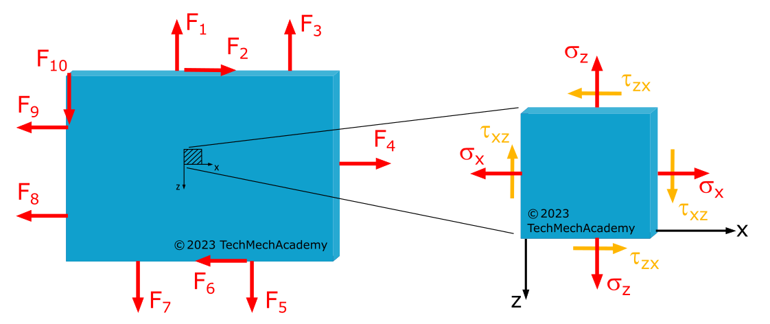
This figure shows the plane stress state.
Fig. 1.3.2: The Plane Stress State for an x, z plane

Another condition for the plane stress state is that the thickness of the component is small relative to its length dimensions, meaning there is a thin wall. Only in this case can we assume that the stresses \(\sigma_x, \sigma_y\), and \(\tau_{xy} = \tau_{yx}\) are uniformly distributed over the entire thickness of the disc.


Not entirely clear about the difference between \(\tau_{xy}\) and \(\tau_{yx}\) or \(\tau_{xz}\) and \(\tau_{zx}\)? Refer to the Index of (Shear) Stresses.

Not entirely clear why \(\tau_{xy} = \tau_{yx}\) or \(\tau_{xz} = \tau_{zx}\)? Refer to the Associated Shear Stresses.

Not entirely clear why the directions of shear stresses differ in Figures 1.3.1 and 1.3.2? Refer to the Determination of Sign for Normal and Shear Stresses.


3.2 Principal Stress

In the previous chapter, we discussed how we can use the given normal and shear stresses (\(\sigma_x\), \(\sigma_y\), and \(\tau_{xy}=\tau_{yx}\) for a vertical section or, alternatively, \(\sigma_x\), \(\sigma_z\), and \(\tau_{xz}=\tau_{zx}\) for an alternately oriented plane) using the transformation equations (1.7xy) and (1.7xz), for calculating normal stresses \(\sigma_{\xi}\) and \(\sigma_{\eta}\) as well as shear stresses \(\tau_{\xi\eta}=\tau_{\eta\xi}\) for any angle of section \(\varphi\).

As a reminder, it's crucial to know at what angle of section \(\varphi\) the largest or smallest stresses act in the examined point of the component and how large they are. This information is essential for making decisions, such as choosing the angles of necessary welds.

The maximum and minimum normal stresses at the examined point of a component are called principal normal stresses or principal stresses. To determine them and the corresponding section angles \(\varphi\), we can do this for two different coordinate systems: once for a Cartesian coordinate system that describes a plane with the x-axis pointing to the right and the y-axis pointing upwards and once for a Cartesian coordinate system describing a plane with the x-axis pointing to the right and the z-axis pointing downwards:

This figure shows a comparison between an x,y coordinate system and an x,z coordinate system, along with the resulting directions of shear stresses.
Fig. 1.3.9: Comparison of the described coordinate systems

We must make this distinction because the direction of shear stresses in the plane depends on the choice of the coordinate system. This is due to the defined sign determination for normal and shear stresses. In practice, knowing the derivation for a preferred coordinate system and being able to calculate its coordinate transformation is sufficient. However, as both systems are frequently used, we will provide both derivations here.

3.2.1 Determination of Principal Stresses for a Cartesian Coordinate System with the Positive x-Axis to the Right and the Positive y-Axis Upward

This figure shows a rotated coordinate system for plane stress state.
Fig. 1.3.10: Determination of Principal Stresses: Rotated Coordinate System for an x, y Plane

We achieve our goal by determining the extreme values of the two equations \(\sigma_{\xi}(\varphi)\) and \(\sigma_{\eta}(\varphi)\) from formula (1.7xy).

This is achieved by taking derivatives of the functions and setting them to zero since at the extreme points of a function, the tangents (= derivative) have no slope (= are zero).

Formula (1.7xy):

$$ \begin{align} \tag{1} \sigma_{\xi} &= \dfrac{1}{2} \cdot \Bigl(\sigma_x + \sigma_y\Bigr) + \dfrac{1}{2} \cdot \Bigl(\sigma_x - \sigma_y\Bigr) \cdot \cos(2\varphi) + \tau_{xy} \cdot \sin(2\varphi) \\[10pt] \tag{2} \sigma_{\eta} &= \dfrac{1}{2} \cdot \Bigl(\sigma_x + \sigma_y\Bigr) - \dfrac{1}{2} \cdot \Bigl(\sigma_x - \sigma_y\Bigr) \cdot \cos(2\varphi) - \tau_{xy} \cdot \sin(2\varphi) \end{align} $$

Thus, we differentiate the functions. Initially, we apply the sum rule:

$$ \begin{align} \tag{3} \dfrac{\mathrm{d}\sigma_{\xi}}{\mathrm{d}\varphi} &= \dfrac{\mathrm{d}}{\mathrm{d}\varphi}\biggl[\dfrac{1}{2} \cdot \Bigl(\sigma_x + \sigma_y\Bigr)\biggr] + \dfrac{\mathrm{d}}{\mathrm{d}\varphi}\biggl[\dfrac{1}{2} \cdot \Bigl(\sigma_x - \sigma_y\Bigr) \cdot \cos(2\varphi)\biggr] + \dfrac{\mathrm{d}}{\mathrm{d}\varphi}\biggl[\tau_{xy} \cdot \sin(2\varphi)\biggr] \\[10pt] \tag{4} \dfrac{\mathrm{d}\sigma_{\eta}}{\mathrm{d}\varphi} &= \dfrac{\mathrm{d}}{\mathrm{d}\varphi}\biggl[\dfrac{1}{2} \cdot \Bigl(\sigma_x + \sigma_y\Bigr)\biggr] - \dfrac{\mathrm{d}}{\mathrm{d}\varphi}\biggl[\dfrac{1}{2} \cdot \Bigl(\sigma_x - \sigma_y\Bigr) \cdot \cos(2\varphi)\biggr] - \dfrac{\mathrm{d}}{\mathrm{d}\varphi}\biggl[\tau_{xy} \cdot \sin(2\varphi)\biggr] \end{align} $$

The first terms in all derivatives are constants, and their derivative is zero:

$$ \begin{align} \tag{5} \dfrac{\mathrm{d}}{\mathrm{d}\varphi}\biggl[\dfrac{1}{2} \cdot \Bigl(\sigma_x + \sigma_y\Bigr)\biggr] = 0 \end{align} $$

For the remaining terms, we apply the multiplication by constant rule to obtain:

$$ \begin{align} \tag{6} \dfrac{\mathrm{d}\sigma_{\xi}}{\mathrm{d}\varphi} &= 0 + \dfrac{1}{2} \cdot \Bigl(\sigma_x - \sigma_y\Bigr) \cdot \dfrac{\mathrm{d}}{\mathrm{d}\varphi}\biggl[\cos(2\varphi)\biggr] + \tau_{xy} \cdot \dfrac{\mathrm{d}}{\mathrm{d}\varphi}\biggl[\sin(2\varphi)\biggr] \\[10pt] \tag{7} \dfrac{\mathrm{d}\sigma_{\eta}}{\mathrm{d}\varphi} &= 0 - \dfrac{1}{2} \cdot \Bigl(\sigma_x - \sigma_y\Bigr) \cdot \dfrac{\mathrm{d}}{\mathrm{d}\varphi}\biggl[\cos(2\varphi)\biggr] - \tau_{xy} \cdot \dfrac{\mathrm{d}}{\mathrm{d}\varphi}\biggl[\sin(2\varphi)\biggr] \end{align} $$

We obtain the derivatives of the trigonometric functions \(\sin\) and \(\cos\) from the table of derivatives of basic functions.

As the argument of these functions is not just \(\varphi\), we also need to apply the chain rule:

$$ \begin{align} \tag{8} \dfrac{\mathrm{d}\sigma_{\xi}}{\mathrm{d}\varphi} &= 0 + \dfrac{1}{2} \cdot \Bigl(\sigma_x - \sigma_y\Bigr) \cdot (-) \sin(2\varphi) \cdot 2 + \tau_{xy} \cdot \cos(2\varphi) \cdot 2 \\[10pt] \tag{9} \dfrac{\mathrm{d}\sigma_{\eta}}{\mathrm{d}\varphi} &= 0 - \dfrac{1}{2} \cdot \Bigl(\sigma_x - \sigma_y\Bigr) \cdot (-) \sin(2\varphi) \cdot 2 - \tau_{xy} \cdot \cos(2\varphi) \cdot 2 \end{align} $$

We thus obtain two derivative functions for the coordinate system \(x, y\) (\(x\) to the right is positive, \(y\) upward is positive), and we set them to zero to find the positions of the extreme values (slope is zero at these points):

$$ \begin{align} \tag{10} \dfrac{\mathrm{d}\sigma_{\xi}}{\mathrm{d}\varphi} &= - \Bigl(\sigma_x - \sigma_y\Bigr) \cdot \sin(2\varphi) + 2 \cdot \tau_{xy} \cdot \cos(2\varphi) = 0 \\[10pt] \tag{11} \dfrac{\mathrm{d}\sigma_{\eta}}{\mathrm{d}\varphi} &= + \Bigl(\sigma_x - \sigma_y\Bigr) \cdot \sin(2\varphi) - 2 \cdot \tau_{xy} \cdot \cos(2\varphi) = 0 \end{align} $$

We divide the equations by \(\cos(2\varphi)\), meaning we divide each term of the equations by \(\cos(2\varphi)\):

$$ \begin{align} \tag{12} \dfrac{\mathrm{d}\sigma_{\xi}}{\mathrm{d}\varphi} &= - \Bigl(\sigma_x - \sigma_y\Bigr) \cdot \dfrac{\sin(2\varphi)}{\cos(2\varphi)} + 2 \cdot \tau_{xy} = 0 \\[10pt] \tag{13} \dfrac{\mathrm{d}\sigma_{\eta}}{\mathrm{d}\varphi} &= + \Bigl(\sigma_x - \sigma_y\Bigr) \cdot \dfrac{\sin(2\varphi)}{\cos(2\varphi)} - 2 \cdot \tau_{xy} = 0 \end{align} $$

Using \(\dfrac{\sin(2\varphi)}{\cos(2\varphi)}= \tan(2\varphi)\), we finalize the equations:

$$ \begin{align} \tag{14} \dfrac{\mathrm{d}\sigma_{\xi}}{\mathrm{d}\varphi} &= - \bigl(\sigma_x - \sigma_y\bigr) \cdot \tan(2\varphi) + 2 \cdot \tau_{xy} = 0 \\[10pt] \tag{15} \dfrac{\mathrm{d}\sigma_{\eta}}{\mathrm{d}\varphi} &= + \bigl(\sigma_x - \sigma_y\bigr) \cdot \tan(2\varphi) - 2 \cdot \tau_{xy} = 0 \end{align} $$

We rearrange both equations to solve for \(\tan(2\varphi)\). To clarify that the angle \(\varphi\) is a specific angle, namely the angle at which the principal normal stresses occur, we call it \(\varphi^*\). In both cases, we have:

$$ \begin{aligned} \tan(2\varphi^*) &= \dfrac{2 \cdot \tau_{xy}}{\sigma_x - \sigma_y} \qquad \Rightarrow \qquad \varphi^* = \dfrac{1}{2}\arctan\Biggl(\dfrac{2 \cdot \tau_{xy}}{\sigma_x - \sigma_y}\Biggr) \end{aligned} $$

Note:

Therefore, we obtain extreme values for the two stresses \(\sigma_{\xi}(\varphi)\) and \(\sigma_{\eta}(\varphi)\) of the coordinate system used for the same angle \(\varphi^*\).

What does this mean in concrete terms?
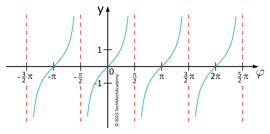
This image shows the tangent function.
Fig. 1.3.11: Tangent Function

The tangent function is periodic with a period of \(\pi\), which means the tangent function has the same value for all \(\varphi\) that differ by \(\pi\).

The argument of the tangent function in the above equation is not simply \(\varphi^*\) but \(2\varphi^*\).

Therefore, here we have:

$$ \begin{align} \tag{16} \tan(2\varphi^*) &= \tan(2\varphi^*\pm\pi) = \tan\biggl(2\Bigl(\varphi^*\pm\dfrac{\pi}{2}\Bigr)\biggr) \end{align} $$

As a reminder, \(\frac{\pi}{2}\) in radians corresponds to \(90°\) in degrees.
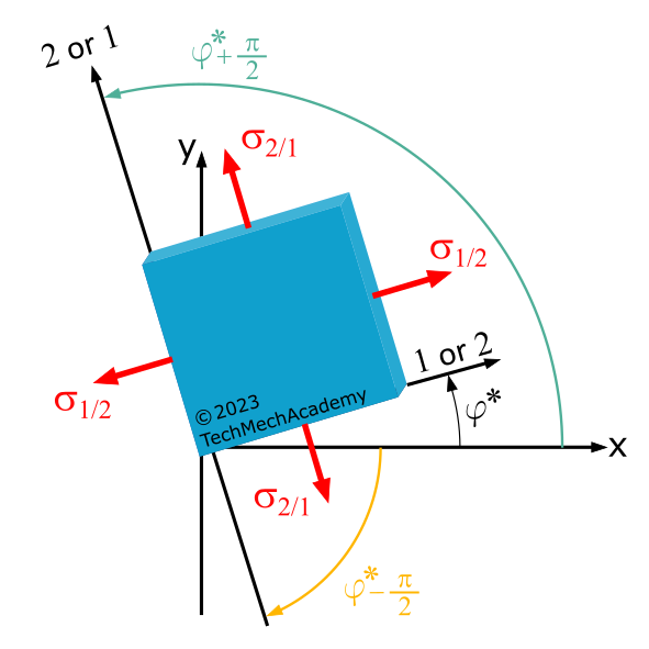
This image shows the cutting angle Phi and the angles phi +90° and phi -90°.
Fig. 1.3.12: Cutting Angles \(\varphi^*\) and \(\varphi^*\pm\frac{\pi}{2}\) in the x,y Coordinate System

Keep in mind that our previous considerations in this chapter apply to an \(x,y\) coordinate system where the positive \(y\) axis is oriented at an angle of \(+\frac{\pi}{2}\) with respect to the \(x\) axis. In concrete terms, this means:

There are two perpendicular cutting directions \(\varphi^*\) and \(\varphi^* + \frac{\pi}{2}\) for which the above equation is satisfied:

$$ \begin{aligned} \tan(2\varphi^*) &= \dfrac{2 \cdot \tau_{xy}}{\sigma_x - \sigma_y} \qquad \Rightarrow \qquad \varphi^* = \dfrac{1}{2}\arctan\Biggl(\dfrac{2 \cdot \tau_{xy}}{\sigma_x - \sigma_y}\Biggr), \qquad \varphi_{II}^* = \varphi^* + \dfrac{\pi}{2} \end{aligned} $$

(1.9xy)

These cutting directions are referred to as principal cutting directions.

Each of the principal cutting directions corresponds to either the maximum or minimum normal stress at the analyzed point in a component.

Since the two principal cutting directions are oriented at an angle of \(\frac{\pi}{2}\) or \(90°\) to each other, there exists a coordinate system with axes parallel to the principal cutting directions.

This coordinate system is referred to as the principal axis system.

We obtain the principal stresses associated with the principal directions by coupling Equation (1.9xy) with Equation (1.7xy).

The coupling is done by initially replacing \(\sin(2\varphi)\) and \(\cos(2\varphi)\) in Equation (1.7xy) with Equation (1.9xy) using the conversions between trigonometric functions.

This results in the following for an \(x,y\)-coordinate system with the positive \(x\) axis to the right and the positive \(y\) axis upwards for \(\sin(2\varphi)_{xy}\):

Show all calculation steps
$$ \begin{align} \tag{17} sin(2\varphi)_{xy} &= \dfrac{\tan(2\varphi^*)}{\sqrt{1+\tan^2(2\varphi^*)}} \qquad \Biggr|~\text{Now insert equation 1.9xy}\Biggl. \\[10pt] \tag{18} &= \dfrac{\dfrac{2 \cdot \tau_{xy}}{\sigma_x-\sigma_y}}{\sqrt{1+\Biggl(\dfrac{2 \cdot \tau_{xy}}{\sigma_x-\sigma_y}\Biggr)^2}} \\[10pt] \tag{19} &= \dfrac{\dfrac{2 \cdot \tau_{xy}}{\sigma_x-\sigma_y}}{\sqrt{\dfrac{(\sigma_x-\sigma_y)^2}{(\sigma_x-\sigma_y)^2}+\dfrac{(2 \cdot \tau_{xy})^2}{(\sigma_x-\sigma_y)^2}}}\\[10pt] \tag{20} &= \dfrac{\tau_{xy}}{\dfrac{\sigma_x-\sigma_y}{2}\sqrt{\dfrac{(\sigma_x-\sigma_y)^2+4 \tau_{xy}^2}{(\sigma_x-\sigma_y)^2} } }\\[10pt] \tag{21} &= \dfrac{\tau_{xy}}{\dfrac{\sigma_x-\sigma_y}{2} \cdot \dfrac{ \sqrt{(\sigma_x-\sigma_y)^2+4 \tau_{xy}^2}}{\sqrt{(\sigma_x-\sigma_y)^2}} }\\[10pt] \tag{22} &= \dfrac{\tau_{xy}}{\dfrac{\sigma_x-\sigma_y}{\sqrt{2^2}} \cdot \dfrac{ \sqrt{(\sigma_x-\sigma_y)^2+4 \tau_{xy}^2}}{\sigma_x-\sigma_y} }\\[10pt] \tag{23} &= \dfrac{\tau_{xy}}{\dfrac{\sqrt{(\sigma_x-\sigma_y)^2+4 \tau_{xy}^2}}{\sqrt{2^2}} } \\[10pt] \tag{24} &= \dfrac{\tau_{xy}}{\sqrt{ \dfrac{(\sigma_x-\sigma_y)^2}{2^2}+ \dfrac{4 \tau_{xy}^2}{2^2} }} \end{align} $$
$$ \begin{align} \tag{25} \sin(2\varphi)_{xy} &= \dfrac{\tau_{xy}}{\sqrt{ \Bigl(\dfrac{\sigma_x-\sigma_y}{2}\Bigr)^2+ \tau_{xy}^2}} \end{align} $$

And for \(\cos(2\varphi)_{xy}\):

Show all calculation steps
$$ \begin{align} \tag{26} \cos(2\varphi)_{xy} &= \dfrac{1}{\sqrt{1+\tan^2(2\varphi^*)}} \qquad \Biggr|~\text{Now insert equation 1.9xy}\Biggl. \\[10pt] \tag{27} &= \dfrac{1}{\sqrt{1+\Biggl(\dfrac{2 \cdot \tau_{xy}}{\sigma_x-\sigma_y}\Biggr)^2}} \\[10pt] \tag{28} &= \dfrac{1}{\sqrt{\dfrac{(\sigma_x-\sigma_y)^2}{(\sigma_x-\sigma_y)^2}+\dfrac{(2 \cdot \tau_{xy})^2}{(\sigma_x-\sigma_y)^2}}} \\[10pt] \tag{29} &= \dfrac{1}{\sqrt{\dfrac{(\sigma_x-\sigma_y)^2+4 \tau_{xy}^2}{(\sigma_x-\sigma_y)^2} } } \\[10pt] \tag{30} &= \dfrac{1}{\dfrac{ \sqrt{(\sigma_x-\sigma_y)^2+4 \tau_{xy}^2}}{\sqrt{(\sigma_x-\sigma_y)^2}} } \\[10pt] \tag{31} &= \dfrac{1}{\dfrac{ \sqrt{(\sigma_x-\sigma_y)^2+4 \tau_{xy}^2}}{\sigma_x-\sigma_y} } \\[10pt] \tag{32} &= \dfrac{\sigma_x-\sigma_y}{\sqrt{(\sigma_x-\sigma_y)^2+4 \tau_{xy}^2}} \\[10pt] \tag{33} &= \dfrac{\dfrac{1}{2} \cdot (\sigma_x-\sigma_y)}{\dfrac{1}{2} \cdot\sqrt{(\sigma_x-\sigma_y)^2+4 \tau_{xy}^2}} \\[10pt] \tag{34} &= \dfrac{\Bigl(\dfrac{\sigma_x-\sigma_y}{2}\Bigr)}{\dfrac{\sqrt{(\sigma_x-\sigma_y)^2+4 \tau_{xy}^2}}{\sqrt{2^2}}} \\[10pt] \tag{35} &= \dfrac{\Bigl(\dfrac{\sigma_x-\sigma_y}{2}\Bigr)}{\sqrt{ \dfrac{(\sigma_x-\sigma_y)^2}{2^2}+ \dfrac{4 \tau_{xy}^2}{2^2} }} \end{align} $$
$$ \begin{align} \tag{36} \cos(2\varphi)_{xy} &= \dfrac{\Bigl(\dfrac{\sigma_x-\sigma_y}{2}\Bigr)}{\sqrt{ \Bigl(\dfrac{\sigma_x-\sigma_y}{2}\Bigr)^2+ \tau_{xy}^2}} \end{align} $$

Now we can determine the principal stresses using Equation (1.7xy) by calculating \(\sigma = \sigma_\xi(\varphi=\varphi^*)\) and \(\sigma = \sigma_\eta(\varphi=\varphi^*)\).

This means for \(\sigma = \sigma_\xi(\varphi=\varphi^*)\):

Show all calculation steps
$$ \begin{align} \tag{37} \sigma &= \sigma_\xi(\varphi=\varphi^*) = \dfrac{1}{2} \cdot \Bigl(\sigma_x + \sigma_y\Bigr) + \dfrac{1}{2} \cdot \Bigl(\sigma_x - \sigma_y\Bigr) \cdot \cos(2\varphi^*) + \tau_{xy} \cdot \sin(2\varphi^*) \\[10pt] \tag{38} \sigma &= \dfrac{1}{2} \cdot \Bigl(\sigma_x + \sigma_y\Bigr) + \dfrac{\dfrac{1}{2} \cdot \Bigl(\sigma_x - \sigma_y\Bigr) \cdot \Bigl(\dfrac{\sigma_x-\sigma_y}{2}\Bigr)}{\sqrt{ \Bigl(\dfrac{\sigma_x-\sigma_y}{2}\Bigr)^2+ \tau_{xy}^2}} + \dfrac{\tau_{xy}\cdot \tau_{xy}}{\sqrt{ \Bigl(\dfrac{\sigma_x-\sigma_y}{2}\Bigr)^2+ \tau_{xy}^2}} \\[10pt] \tag{39} \sigma &= \dfrac{1}{2} \cdot \Bigl(\sigma_x + \sigma_y\Bigr) + \dfrac{\Bigl(\dfrac{\sigma_x-\sigma_y}{2}\Bigr) \cdot \Bigl(\dfrac{\sigma_x-\sigma_y}{2}\Bigr) + \tau_{xy}^2}{\sqrt{\Bigl(\dfrac{\sigma_x-\sigma_y}{2}\Bigr)^2+ \tau_{xy}^2}} \\[10pt] \tag{40} \sigma &= \dfrac{1}{2} \cdot \Bigl(\sigma_x + \sigma_y\Bigr) + \dfrac{\Bigl(\dfrac{\sigma_x-\sigma_y}{2}\Bigr)^2 + \tau_{xy}^2}{\sqrt{\Bigl(\dfrac{\sigma_x-\sigma_y}{2}\Bigr)^2+ \tau_{xy}^2}} \end{align} $$

Using the exponent rules for powers with the same base,

$$ \begin{align} \tag{41} \dfrac{a^m}{a^n} &= a^{m-n} \end{align} $$

and considering the radical rules

$$ \begin{align} \tag{42} \sqrt[n]{a}&=a^{\frac{1}{n}} \\[7pt] \tag{43} \sqrt[2]{a}&=\sqrt{a} \end{align} $$

we obtain:

$$ \begin{align} \tag{44} \sigma &= \dfrac{1}{2} \cdot \Bigl(\sigma_x + \sigma_y\Bigr) + \dfrac{\biggl(\Bigl(\dfrac{\sigma_x-\sigma_y}{2}\Bigr)^2 + \tau_{xy}^2\biggr)^1}{\biggl(\Bigl(\dfrac{\sigma_x-\sigma_y}{2}\Bigr)^2+ \tau_{xy}^2\biggr)^{\frac{1}{2}}} \\[10pt] \tag{45} \sigma &= \dfrac{1}{2} \cdot \Bigl(\sigma_x + \sigma_y\Bigr) + \biggl(\Bigl(\dfrac{\sigma_x-\sigma_y}{2}\Bigr)^2+ \tau_{xy}^2\biggr)^{1-\frac{1}{2}} \end{align} $$
$$ \begin{aligned} \sigma &= \dfrac{1}{2} \cdot \Bigl(\sigma_x + \sigma_y\Bigr) + \sqrt{\Bigl(\dfrac{\sigma_x-\sigma_y}{2}\Bigr)^2+ \tau_{xy}^2} \end{aligned} $$

This is a formula for one of the principal stresses

If we want to determine the principal stress through the calculation of \(\sigma = \sigma_\eta(\varphi=\varphi^*)\), it means:

Show all calculation steps
$$ \begin{align} \tag{46} \sigma &= \sigma_\eta(\varphi=\varphi^*) = \dfrac{1}{2} \cdot \Bigl(\sigma_x + \sigma_y\Bigr) - \dfrac{1}{2} \cdot \Bigl(\sigma_x - \sigma_y\Bigr) \cdot \cos(2\varphi^*) - \tau_{xy} \cdot \sin(2\varphi^*) \\[10pt] \tag{47} \sigma &= \dfrac{1}{2} \cdot \Bigl(\sigma_x + \sigma_y\Bigr) - \dfrac{\dfrac{1}{2} \cdot \Bigl(\sigma_x - \sigma_y\Bigr) \cdot \Bigl(\dfrac{\sigma_x-\sigma_y}{2}\Bigr)}{\sqrt{ \Bigl(\dfrac{\sigma_x-\sigma_y}{2}\Bigr)^2+ \tau_{xy}^2}} - \dfrac{\tau_{xy}\cdot \tau_{xy}}{\sqrt{ \Bigl(\dfrac{\sigma_x-\sigma_y}{2}\Bigr)^2+ \tau_{xy}^2}} \\[10pt] \tag{48} \sigma &= \dfrac{1}{2} \cdot \Bigl(\sigma_x + \sigma_y\Bigr) - \left[\dfrac{\dfrac{1}{2} \cdot \Bigl(\sigma_x - \sigma_y\Bigr) \cdot \Bigl(\dfrac{\sigma_x-\sigma_y}{2}\Bigr)}{\sqrt{ \Bigl(\dfrac{\sigma_x-\sigma_y}{2}\Bigr)^2+ \tau_{xy}^2}} + \dfrac{\tau_{xy}\cdot \tau_{xy}}{\sqrt{ \Bigl(\dfrac{\sigma_x-\sigma_y}{2}\Bigr)^2+ \tau_{xy}^2}}\right] \\[10pt] \tag{49} \sigma &= \dfrac{1}{2} \cdot \Bigl(\sigma_x + \sigma_y\Bigr) - \dfrac{\Bigl(\dfrac{\sigma_x-\sigma_y}{2}\Bigr) \cdot \Bigl(\dfrac{\sigma_x-\sigma_y}{2}\Bigr) + \tau_{xy}^2}{\sqrt{\Bigl(\dfrac{\sigma_x-\sigma_y}{2}\Bigr)^2+ \tau_{xy}^2}} \\[10pt] \tag{50} \sigma &= \dfrac{1}{2} \cdot \Bigl(\sigma_x + \sigma_y\Bigr) - \dfrac{\Bigl(\dfrac{\sigma_x-\sigma_y}{2}\Bigr)^2 + \tau_{xy}^2}{\sqrt{\Bigl(\dfrac{\sigma_x-\sigma_y}{2}\Bigr)^2+ \tau_{xy}^2}} \end{align} $$

Using the exponent rules for powers with the same base,

$$ \begin{align} \tag{51} \dfrac{a^m}{a^n} &= a^{m-n} \end{align} $$

and considering the radical rules

$$ \begin{align} \tag{52} \sqrt[n]{a}&=a^{\frac{1}{n}} \\[7pt] \tag{53} \sqrt[2]{a}&=\sqrt{a} \end{align} $$

we obtain:

$$ \begin{align} \tag{54} \sigma &= \dfrac{1}{2} \cdot \Bigl(\sigma_x + \sigma_y\Bigr) - \dfrac{\biggl(\Bigl(\dfrac{\sigma_x-\sigma_y}{2}\Bigr)^2 + \tau_{xy}^2\biggr)^1}{\biggl(\Bigl(\dfrac{\sigma_x-\sigma_y}{2}\Bigr)^2 + \tau_{xy}^2\biggr)^{\frac{1}{2}}} \\[10pt] \tag{55} \sigma &= \dfrac{1}{2} \cdot \Bigl(\sigma_x + \sigma_y\Bigr) - \biggl(\Bigl(\dfrac{\sigma_x-\sigma_y}{2}\Bigr)^2 + \tau_{xy}^2\biggr)^{1-\frac{1}{2}} \end{align} $$
$$ \begin{aligned} \sigma &= \dfrac{1}{2} \cdot \Bigl(\sigma_x + \sigma_y\Bigr) - \sqrt{\Bigl(\dfrac{\sigma_x-\sigma_y}{2}\Bigr)^2 + \tau_{xy}^2} \end{aligned} $$

This is a formula for one of the principal stresses

The question remains, how large the shear stresses are under the principal shear directions \(\varphi^*\) and \(\varphi_{II}^*\).

Let's substitute the values we derived above:

$$ \begin{align} \tag{56} \sin(2\varphi)_{xy} &= \dfrac{\tau_{xy}}{\sqrt{ \Bigl(\dfrac{\sigma_x-\sigma_y}{2}\Bigr)^2+ \tau_{xy}^2}} \end{align} $$

and

$$ \begin{align} \tag{57} \cos(2\varphi)_{xy} &= \dfrac{\Bigl(\dfrac{\sigma_x-\sigma_y}{2}\Bigr)}{\sqrt{ \Bigl(\dfrac{\sigma_x-\sigma_y}{2}\Bigr)^2+ \tau_{xy}^2}} \end{align} $$

into the equation for \(\tau_{\xi\eta}\) according to (1.7xy), we get:

$$ \begin{align} \tag{58} \tau &= \tau_{\xi\eta}(\varphi=\varphi^*) = - \dfrac{1}{2} \cdot \Bigl(\sigma_x - \sigma_y\Bigr) \cdot \sin(2\varphi) + \tau_{xy} \cdot \cos(2\varphi) \\[10pt] \tag{59} \tau &= - \dfrac{\dfrac{1}{2} \cdot \Bigl(\sigma_x - \sigma_y\Bigr) \cdot \tau_{xy} }{\sqrt{ \Bigl(\dfrac{\sigma_x-\sigma_y}{2}\Bigr)^2+ \tau_{xy}^2}} + \dfrac{\tau_{xy}\cdot \Bigl(\dfrac{\sigma_x-\sigma_y}{2}\Bigr)}{\sqrt{ \Bigl(\dfrac{\sigma_x-\sigma_y}{2}\Bigr)^2+ \tau_{xy}^2}} \\[10pt] \tag{60} \tau &= 0 \end{align} $$

This means:

The shear stresses vanish in the principal shear directions where the normal stresses take extreme values!

In summary, for a Cartesian coordinate system that describes a plane where the x-axis points to the right and the y-axis points upwards, the equations for the principal stresses of the plane stress state are as follows:

$$ \begin{aligned} \sigma_{1,2} &= \dfrac{1}{2} \cdot \Bigl(\sigma_x + \sigma_y\Bigr) \pm \sqrt{\Bigl(\dfrac{\sigma_x-\sigma_y}{2}\Bigr)^2 + \tau_{xy}^2}\\[7pt] &\qquad\text{where}\\[7pt] \tau_{12} &= \tau_{21} = 0 \end{aligned} $$

(1.10xy)

The principal stresses can be positive or negative, depending on whether they indicate tension or compression. The indices of the principal stresses are chosen so that they are sorted in descending order of magnitude, starting with the largest principal stress. So it holds that:

$$ \begin{align} \tag{61} \sigma_1 &> \sigma_2 \end{align} $$

Note:

The angles \(\varphi^*\) and \(\varphi_{II}^*\) calculated using Equation (1.9xy) should not be assigned to the principal stresses \(\sigma_1\) and \(\sigma_2\) based on their indices! The angle \(\varphi^*\) can be either the direction angle between the \(x\)-axis and the first or the second principal stress direction (see Figure 1.3.12).

The assignment of the two angles \(\varphi^*\) and \(\varphi_{II}^* = \varphi^*+\frac{\pi}{2}\) to the principal stresses \(\sigma_1\) and \(\sigma_2\) is usually done by inserting the angle \(\varphi^*\) into the first equation for \(\sigma_\xi\) in Equation (1.7xy).

The calculated normal stress is either \(\sigma_1\) or \(\sigma_2\), and you have found the shear direction associated with this normal stress \(\varphi_1^* = \varphi^*\) or \(\varphi_2^* = \varphi^*\).

Example 1.2: Determining the Magnitude and Direction of Principal Stresses

Let's consider a sheet with the given stresses \(\sigma_x = 20\mathrm{~MPa}\), \(\sigma_y = 30\mathrm{~MPa}\), and \(\tau_{xy} = 10\mathrm{~MPa}\).
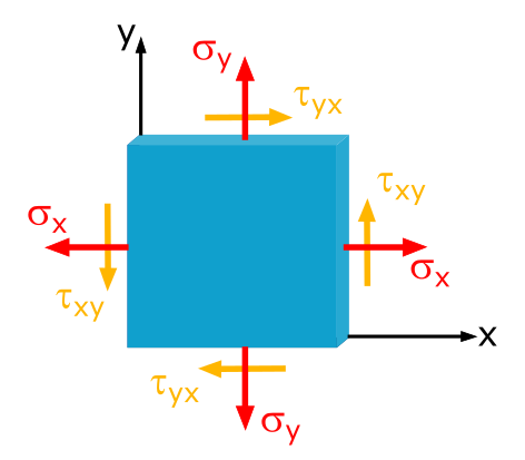
Sheet with given stresses.
Fig. B1.2: Sheet with Given Stresses

Determine the magnitude and direction of the principal stresses.

Solution

For the given \(x\), \(y\)-coordinate system describing a plane where the x-axis points to the right in the positive direction and the y-axis points upward in the positive direction, and the given stresses \(\sigma_x\), \(\sigma_y\), and \(\tau_{xy}\), we can use formula 1.10xy to determine the principal stresses:

Continue with TechMechAcademy+

Everything. Always. Everywhere.

With TechMechAcademy+ full access to all content.

alt
alt
alt
alt
alt

Are you already a TechMechAcademy+ premium member? Then please log in here to enjoy full access to all content.

3.2.2 Determination of Principal Stresses for a Cartesian Coordinate System with Positive x-Axis to the Right and Positive z-Axis Downwards

This figure shows a rotated coordinate system for the planar stress state.
Fig. 1.3.13: Determination of Principal Normal Stresses: Rotated Coordinate System for an x, z Plane

We achieve our goal by determining the extreme values of the two equations \(\sigma_{\xi}(\varphi)\) and \(\sigma_{\eta}(\varphi)\) from formula (1.7xz).

This is achieved by taking derivatives of the functions and setting them to zero since at the extreme points of a function, the tangents (= derivative) have no slope (= are zero).

Formula (1.7xz):

$$ \begin{align} \tag{62} \sigma_{\xi} &= \dfrac{1}{2} \cdot \Bigl(\sigma_x + \sigma_z\Bigr) + \dfrac{1}{2} \cdot \Bigl(\sigma_x - \sigma_z\Bigr) \cdot \cos(2\varphi) - \tau_{xz} \cdot \sin(2\varphi) \\[10pt] \tag{63} \sigma_{\eta} &= \dfrac{1}{2} \cdot \Bigl(\sigma_x + \sigma_z\Bigr) - \dfrac{1}{2} \cdot \Bigl(\sigma_x - \sigma_z\Bigr) \cdot \cos(2\varphi) + \tau_{xz} \cdot \sin(2\varphi) \end{align} $$

Thus, we differentiate the functions. Initially, we apply the sum rule:

$$ \begin{align} \tag{64} \dfrac{\mathrm{d}\sigma_{\xi}}{\mathrm{d}\varphi} &= \dfrac{\mathrm{d}}{\mathrm{d}\varphi}\biggl[\dfrac{1}{2} \cdot \Bigl(\sigma_x + \sigma_z\Bigr)\biggr] + \dfrac{\mathrm{d}}{\mathrm{d}\varphi}\biggl[\dfrac{1}{2} \cdot \Bigl(\sigma_x - \sigma_z\Bigr) \cdot \cos(2\varphi)\biggr] - \dfrac{\mathrm{d}}{\mathrm{d}\varphi}\biggl[\tau_{xz} \cdot \sin(2\varphi)\biggr] \\[10pt] \tag{65} \dfrac{\mathrm{d}\sigma_{\eta}}{\mathrm{d}\varphi} &= \dfrac{\mathrm{d}}{\mathrm{d}\varphi}\biggl[\dfrac{1}{2} \cdot \Bigl(\sigma_x + \sigma_z\Bigr)\biggr] - \dfrac{\mathrm{d}}{\mathrm{d}\varphi}\biggl[\dfrac{1}{2} \cdot \Bigl(\sigma_x - \sigma_z\Bigr) \cdot \cos(2\varphi)\biggr] + \dfrac{\mathrm{d}}{\mathrm{d}\varphi}\biggl[\tau_{xz} \cdot \sin(2\varphi)\biggr] \end{align} $$

The first terms in all derivatives are constants, and their derivative is zero:

$$ \begin{align} \tag{66} \dfrac{\mathrm{d}}{\mathrm{d}\varphi}\biggl[\dfrac{1}{2} \cdot \Bigl(\sigma_x + \sigma_z\Bigr)\biggr] = 0 \end{align} $$

For the remaining terms, we apply the multiplication by constant rule to obtain:

$$ \begin{align} \tag{67} \dfrac{\mathrm{d}\sigma_{\xi}}{\mathrm{d}\varphi} &= 0 + \dfrac{1}{2} \cdot \Bigl(\sigma_x - \sigma_z\Bigr) \cdot \dfrac{\mathrm{d}}{\mathrm{d}\varphi}\biggl[\cos(2\varphi)\biggr] - \tau_{xz} \cdot \dfrac{\mathrm{d}}{\mathrm{d}\varphi}\biggl[\sin(2\varphi)\biggr] \\[10pt] \tag{68} \dfrac{\mathrm{d}\sigma_{\eta}}{\mathrm{d}\varphi} &= 0 - \dfrac{1}{2} \cdot \Bigl(\sigma_x - \sigma_z\Bigr) \cdot \dfrac{\mathrm{d}}{\mathrm{d}\varphi}\biggl[\cos(2\varphi)\biggr] + \tau_{xz} \cdot \dfrac{\mathrm{d}}{\mathrm{d}\varphi}\biggl[\sin(2\varphi)\biggr] \end{align} $$

We obtain the derivatives of the trigonometric functions \(\sin\) and \(\cos\) from the table of derivatives of basic functions.

As the argument of these functions is not just \(\varphi\), we also need to apply the chain rule:

$$ \begin{align} \tag{69} \dfrac{\mathrm{d}\sigma_{\xi}}{\mathrm{d}\varphi} &= 0 + \dfrac{1}{2} \cdot \Bigl(\sigma_x - \sigma_z\Bigr) \cdot (-) \sin(2\varphi) \cdot 2 - \tau_{xz} \cdot \cos(2\varphi) \cdot 2 \\[10pt] \tag{70} \dfrac{\mathrm{d}\sigma_{\eta}}{\mathrm{d}\varphi} &= 0 - \dfrac{1}{2} \cdot \Bigl(\sigma_x - \sigma_z\Bigr) \cdot (-) \sin(2\varphi) \cdot 2 + \tau_{xz} \cdot \cos(2\varphi) \cdot 2 \end{align} $$

We now have two derivative functions for the coordinate system \(x,z\) (\(x\) to the right is positive, \(z\) downwards is positive). To find the locations of the extreme values (where the slope is zero), we set these derivative functions to zero:

$$ \begin{align} \tag{71} \dfrac{\mathrm{d}\sigma_{\xi}}{\mathrm{d}\varphi} &= - \Bigl(\sigma_x - \sigma_z\Bigr) \cdot \sin(2\varphi) - 2 \cdot \tau_{xz} \cdot \cos(2\varphi) = 0 \\[10pt] \tag{72} \dfrac{\mathrm{d}\sigma_{\eta}}{\mathrm{d}\varphi} &= + \Bigl(\sigma_x - \sigma_z\Bigr) \cdot \sin(2\varphi) + 2 \cdot \tau_{xz} \cdot \cos(2\varphi) = 0 \end{align} $$

We divide the equations by \(\cos(2\varphi)\), meaning we divide each term in the equations by \(\cos(2\varphi)\):

$$ \begin{align} \tag{73} \dfrac{\mathrm{d}\sigma_{\xi}}{\mathrm{d}\varphi} &= - \Bigl(\sigma_x - \sigma_z\Bigr) \cdot \dfrac{\sin(2\varphi)}{\cos(2\varphi)} - 2 \cdot \tau_{xz} = 0 \\[10pt] \tag{74} \dfrac{\mathrm{d}\sigma_{\eta}}{\mathrm{d}\varphi} &= + \Bigl(\sigma_x - \sigma_z\Bigr) \cdot \dfrac{\sin(2\varphi)}{\cos(2\varphi)} + 2 \cdot \tau_{xz} = 0 \end{align} $$

Using \(\dfrac{\sin(2\varphi)}{\cos(2\varphi)}= \tan(2\varphi)\), we finalize the equations:

$$ \begin{align} \tag{75} \dfrac{\mathrm{d}\sigma_{\xi}}{\mathrm{d}\varphi} &= - \bigl(\sigma_x - \sigma_z\bigr) \cdot \tan(2\varphi) - 2 \cdot \tau_{xz} = 0 \\[10pt] \tag{76} \dfrac{\mathrm{d}\sigma_{\eta}}{\mathrm{d}\varphi} &= + \bigl(\sigma_x - \sigma_z\bigr) \cdot \tan(2\varphi) + 2 \cdot \tau_{xz} = 0 \end{align} $$

We solve both equations for \(\tan(2\varphi)\). To make it clear that the angle \(\varphi\) is a specific angle, namely the angle at which the principal normal stresses occur, we call it \(\varphi^*\). In both cases, we get:

$$ \begin{aligned} \tan(2\varphi^*) &= -\dfrac{2 \cdot \tau_{xz}}{\sigma_x - \sigma_z} \qquad \Rightarrow \qquad \varphi^* = \dfrac{1}{2}\arctan\Biggl(-\dfrac{2 \cdot \tau_{xz}}{\sigma_x - \sigma_z}\Biggr) \end{aligned} $$

Note:

We thus obtain for the two stresses \(\sigma_{\xi}(\varphi)\) and \(\sigma_{\eta}(\varphi)\) of the used coordinate system extreme values for the same cutting angle \(\varphi^*\).

What does this mean in concrete terms?

This figure shows the tangent function.
Fig. 1.3.14: Tangent Function

The tangent function is periodic with a period of \(\pi\). In other words, the tangent function has the same value for all \(\varphi\) values that differ by \(\pi\).

The argument of the tangent function in the above equation is not simply \(\varphi^*\) but \(2\varphi^*\).

Therefore, the following holds here:

$$ \begin{align} \tag{77} \tan(2\varphi^*) &= \tan(2\varphi^*\pm\pi) = \tan\biggl(2\Bigl(\varphi^*\pm\dfrac{\pi}{2}\Bigr)\biggr) \end{align} $$

As a reminder, \(\frac{\pi}{2}\) in radians corresponds to \(90°\) in degrees.
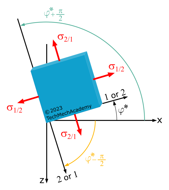
This figure shows the cutting angle \(\varphi^*\) and \(\varphi^*\pm\dfrac{\pi}{2}\) in the x,z coordinate system.
Fig. 1.3.15: Cutting Angles \(\varphi^*\) and \(\varphi^*\pm\dfrac{\pi}{2}\) in the x,z Coordinate System

Let's note that our previous considerations in this chapter apply to an \(x,z\) coordinate system where the positive \(z\)-axis is oriented at an angle of \(-\frac{\pi}{2}\) with respect to the \(x\)-axis. This means concretely:

There are two mutually perpendicular cutting directions \(\varphi^*\) and \(\varphi^* - \dfrac{\pi}{2}\) for which the above equation is satisfied:

$$ \begin{aligned} \tan(2\varphi^*) &= -\dfrac{2 \cdot \tau_{xz}}{\sigma_x - \sigma_z} \qquad \Rightarrow \qquad \varphi^* = \dfrac{1}{2}\arctan\Biggl(-\dfrac{2 \cdot \tau_{xz}}{\sigma_x - \sigma_z}\Biggr), \qquad \varphi_{II}^* = \varphi^* - \dfrac{\pi}{2} \end{aligned} $$

(1.9xz)

Note:

At some universities, similar to calculating the principal stress directions in the \(x,y\) coordinate system, it is preferred to calculate \(\varphi_{II}^* = \varphi^* \mathbf{+} \dfrac{\pi}{2}\). This cutting direction is essentially equivalent to the cutting direction \(\varphi_{II}^* = \varphi^* \mathbf{-} \dfrac{\pi}{2}\) since they both describe the same principal stress direction as shown in Figure 1.3.15.

These cutting directions are referred to as principal stress directions.

Each of the two principal stress directions corresponds to either the maximum or minimum normal stress at the examined point of a component.

Since the two principal stress directions are oriented at an angle of \(\frac{\pi}{2}\) or \(90°\) to each other, there exists a coordinate system with its axes parallel to the principal stress directions.

This coordinate system is referred to as the principal axis system.

We obtain the principal stresses associated with the principal directions by coupling equation (1.9xz) with equation (1.7xz).

The coupling is achieved by initially replacing \(\sin(2\varphi)\) and \(\cos(2\varphi)\) from equation (1.7xy) with equation (1.9xz) using the conversions between trigonometric functions.

This results in the following for an \(x,z\) coordinate system with the positive \(x\)-axis to the right and the positive \(z\)-axis downward for \(\sin(2\varphi)_{xz}\):

Show all calculation steps
$$ \begin{align} \tag{78} \sin(2\varphi)_{xz} &= \dfrac{\tan(2\varphi^*)}{\sqrt{1+\tan^2(2\varphi^*)}} \qquad \Biggr|~\text{Now substitute equation 1.9xz}\Biggl. \\[10pt] \tag{79} &= \dfrac{-\dfrac{2 \cdot \tau_{xz}}{\sigma_x-\sigma_z}}{\sqrt{1+\Biggl(-\dfrac{2 \cdot \tau_{xz}}{\sigma_x-\sigma_z}\Biggr)^2}} \\[10pt] \tag{80} &= \dfrac{-\dfrac{2 \cdot \tau_{xz}}{\sigma_x-\sigma_z}}{\sqrt{\dfrac{(\sigma_x-\sigma_z)^2}{(\sigma_x-\sigma_z)^2}+\dfrac{(-2 \cdot \tau_{xz})^2}{(\sigma_x-\sigma_z)^2}}}\\[10pt] \tag{81} &= \dfrac{-\tau_{xz}}{\dfrac{\sigma_x-\sigma_z}{2}\sqrt{\dfrac{(\sigma_x-\sigma_z)^2+4 \tau_{xz}^2}{(\sigma_x-\sigma_z)^2} } }\\[10pt] \tag{82} &= -\dfrac{\tau_{xz}}{\dfrac{\sigma_x-\sigma_z}{2} \cdot \dfrac{ \sqrt{(\sigma_x-\sigma_z)^2+4 \tau_{xz}^2}}{\sqrt{(\sigma_x-\sigma_z)^2}} }\\[10pt] \tag{83} &= -\dfrac{\tau_{xz}}{\dfrac{\sigma_x-\sigma_z}{\sqrt{2^2}} \cdot \dfrac{ \sqrt{(\sigma_x-\sigma_z)^2+4 \tau_{xz}^2}}{\sigma_x-\sigma_z} }\\[10pt] \tag{84} &= -\dfrac{\tau_{xz}}{\dfrac{\sqrt{(\sigma_x-\sigma_z)^2+4 \tau_{xz}^2}}{\sqrt{2^2}} } \\[10pt] \tag{85} &= -\dfrac{\tau_{xz}}{\sqrt{ \dfrac{(\sigma_x-\sigma_z)^2}{2^2}+ \dfrac{4 \tau_{xz}^2}{2^2} }} \end{align} $$
$$ \begin{align} \tag{86} \sin(2\varphi)_{xz} &= -\dfrac{\tau_{xz}}{\sqrt{ \Bigl(\dfrac{\sigma_x-\sigma_z}{2}\Bigr)^2+ \tau_{xz}^2}} \end{align} $$

And for \(\cos(2\varphi)_{xz}\):

Show all calculation steps
$$ \begin{align} \tag{87} \cos(2\varphi)_{xz} &= \dfrac{1}{\sqrt{1+\tan^2(2\varphi^*)}} \qquad \Biggr|~\text{Now substitute equation 1.9xz}\Biggl. \\[10pt] \tag{88} &= \dfrac{1}{\sqrt{1+\Biggl(-\dfrac{2 \cdot \tau_{xz}}{\sigma_x-\sigma_z}\Biggr)^2}} \\[10pt] \tag{89} &= \dfrac{1}{\sqrt{\dfrac{(\sigma_x-\sigma_z)^2}{(\sigma_x-\sigma_z)^2}+\dfrac{(-2 \cdot \tau_{xz})^2}{(\sigma_x-\sigma_z)^2}}} \\[10pt] \tag{90} &= \dfrac{1}{\sqrt{\dfrac{(\sigma_x-\sigma_z)^2+4 \tau_{xz}^2}{(\sigma_x-\sigma_z)^2} } } \\[10pt] \tag{91} &= \dfrac{1}{\dfrac{ \sqrt{(\sigma_x-\sigma_z)^2+4 \tau_{xz}^2}}{\sqrt{(\sigma_x-\sigma_z)^2}} } \\[10pt] \tag{92} &= \dfrac{1}{\dfrac{ \sqrt{(\sigma_x-\sigma_z)^2+4 \tau_{xz}^2}}{\sigma_x-\sigma_z} } \\[10pt] \tag{93} &= \dfrac{\sigma_x-\sigma_z}{\sqrt{(\sigma_x-\sigma_z)^2+4 \tau_{xz}^2}} \\[10pt] \tag{94} &= \dfrac{\dfrac{1}{2} \cdot (\sigma_x-\sigma_z)}{\dfrac{1}{2} \cdot\sqrt{(\sigma_x-\sigma_z)^2+4 \tau_{xz}^2}} \\[10pt] \tag{95} &= \dfrac{\Bigl(\dfrac{\sigma_x-\sigma_z}{2}\Bigr)}{\dfrac{\sqrt{(\sigma_x-\sigma_z)^2+4 \tau_{xz}^2}}{\sqrt{2^2}}} \\[10pt] \tag{96} &= \dfrac{\Bigl(\dfrac{\sigma_x-\sigma_z}{2}\Bigr)}{\sqrt{ \dfrac{(\sigma_x-\sigma_z)^2}{2^2}+ \dfrac{4 \tau_{xz}^2}{2^2} }} \end{align} $$
$$ \begin{align} \tag{97} \cos(2\varphi)_{xz} &= \dfrac{\Bigl(\dfrac{\sigma_x-\sigma_z}{2}\Bigr)}{\sqrt{ \Bigl(\dfrac{\sigma_x-\sigma_z}{2}\Bigr)^2+ \tau_{xz}^2}} \end{align} $$

Now we can determine the principal stresses using equation (1.7xz) by calculating \(\sigma = \sigma_\xi(\varphi=\varphi^*)\) and \(\sigma = \sigma_\eta(\varphi=\varphi^*)\).

This means for \(\sigma = \sigma_\xi(\varphi=\varphi^*)\):

Show all calculation steps
$$ \begin{align} \tag{98} \sigma &= \sigma_\xi(\varphi=\varphi^*) = \dfrac{1}{2} \cdot \Bigl(\sigma_x + \sigma_z\Bigr) + \dfrac{1}{2} \cdot \Bigl(\sigma_x - \sigma_z\Bigr) \cdot \cos(2\varphi^*) - \tau_{xz} \cdot \sin(2\varphi^*) \\[10pt] \tag{99} \sigma &= \dfrac{1}{2} \cdot \Bigl(\sigma_x + \sigma_z\Bigr) + \dfrac{\dfrac{1}{2} \cdot \Bigl(\sigma_x - \sigma_z\Bigr) \cdot \Bigl(\dfrac{\sigma_x-\sigma_z}{2}\Bigr)}{\sqrt{ \Bigl(\dfrac{\sigma_x-\sigma_z}{2}\Bigr)^2+ \tau_{xz}^2}} - \dfrac{\tau_{xz}\cdot (-)\tau_{xz}}{\sqrt{ \Bigl(\dfrac{\sigma_x-\sigma_z}{2}\Bigr)^2+ \tau_{xz}^2}} \\[10pt] \tag{100} \sigma &= \dfrac{1}{2} \cdot \Bigl(\sigma_x + \sigma_z\Bigr) + \dfrac{\Bigl(\dfrac{\sigma_x-\sigma_z}{2}\Bigr) \cdot \Bigl(\dfrac{\sigma_x-\sigma_z}{2}\Bigr) + \tau_{xz}^2}{\sqrt{\Bigl(\dfrac{\sigma_x-\sigma_z}{2}\Bigr)^2+ \tau_{xz}^2}} \\[10pt] \tag{101} \sigma &= \dfrac{1}{2} \cdot \Bigl(\sigma_x + \sigma_z\Bigr) + \dfrac{\Bigl(\dfrac{\sigma_x-\sigma_z}{2}\Bigr)^2 + \tau_{xz}^2}{\sqrt{\Bigl(\dfrac{\sigma_x-\sigma_z}{2}\Bigr)^2+ \tau_{xz}^2}} \end{align} $$

Using the exponent rules for powers with the same base,

$$ \begin{align} \tag{102} \dfrac{a^m}{a^n} &= a^{m-n} \end{align} $$

and considering the radical rules

$$ \begin{align} \tag{103} \sqrt[n]{a}&=a^{\frac{1}{n}} \\[7pt] \tag{104} \sqrt[2]{a}&=\sqrt{a} \end{align} $$

we obtain:

$$ \begin{align} \tag{105} \sigma &= \dfrac{1}{2} \cdot \Bigl(\sigma_x + \sigma_z\Bigr) + \dfrac{\biggl(\Bigl(\dfrac{\sigma_x-\sigma_z}{2}\Bigr)^2 + \tau_{xz}^2\biggr)^1}{\biggl(\Bigl(\dfrac{\sigma_x-\sigma_z}{2}\Bigr)^2+ \tau_{xz}^2\biggr)^{\frac{1}{2}}} \\[10pt] \tag{106} \sigma &= \dfrac{1}{2} \cdot \Bigl(\sigma_x + \sigma_z\Bigr) + \biggl(\Bigl(\dfrac{\sigma_x-\sigma_z}{2}\Bigr)^2+ \tau_{xz}^2\biggr)^{1-\frac{1}{2}} \end{align} $$
$$ \begin{aligned} \sigma &= \dfrac{1}{2} \cdot \Bigl(\sigma_x + \sigma_z\Bigr) + \sqrt{\Bigl(\dfrac{\sigma_x-\sigma_z}{2}\Bigr)^2+ \tau_{xz}^2} \end{aligned} $$

This is a formula for one of the principal stresses

If we want to determine the principal stress by calculating \(\sigma = \sigma_\eta(\varphi=\varphi^*)\), it means:

Show all calculation steps
$$ \begin{align} \tag{107} \sigma &= \sigma_\eta(\varphi=\varphi^*) = \dfrac{1}{2} \cdot \Bigl(\sigma_x + \sigma_z\Bigr) - \dfrac{1}{2} \cdot \Bigl(\sigma_x - \sigma_z\Bigr) \cdot \cos(2\varphi^*) + \tau_{xz} \cdot \sin(2\varphi^*) \\[10pt] \tag{108} \sigma &= \dfrac{1}{2} \cdot \Bigl(\sigma_x + \sigma_z\Bigr) - \dfrac{\dfrac{1}{2} \cdot \Bigl(\sigma_x - \sigma_z\Bigr) \cdot \Bigl(\dfrac{\sigma_x-\sigma_z}{2}\Bigr)}{\sqrt{ \Bigl(\dfrac{\sigma_x-\sigma_z}{2}\Bigr)^2+ \tau_{xz}^2}} + \dfrac{\tau_{xz}\cdot (-)\tau_{xz}}{\sqrt{ \Bigl(\dfrac{\sigma_x-\sigma_z}{2}\Bigr)^2+ \tau_{xz}^2}} \\[10pt] \tag{109} \sigma &= \dfrac{1}{2} \cdot \Bigl(\sigma_x + \sigma_z\Bigr) - \dfrac{\dfrac{1}{2} \cdot \Bigl(\sigma_x - \sigma_z\Bigr) \cdot \Bigl(\dfrac{\sigma_x-\sigma_z}{2}\Bigr)}{\sqrt{ \Bigl(\dfrac{\sigma_x-\sigma_z}{2}\Bigr)^2+ \tau_{xz}^2}} - \dfrac{\tau_{xz}\cdot \tau_{xz}}{\sqrt{ \Bigl(\dfrac{\sigma_x-\sigma_z}{2}\Bigr)^2+ \tau_{xz}^2}} \\[10pt] \tag{110} \sigma &= \dfrac{1}{2} \cdot \Bigl(\sigma_x + \sigma_z\Bigr) - \left[\dfrac{\dfrac{1}{2} \cdot \Bigl(\sigma_x - \sigma_z\Bigr) \cdot \Bigl(\dfrac{\sigma_x-\sigma_z}{2}\Bigr)}{\sqrt{ \Bigl(\dfrac{\sigma_x-\sigma_z}{2}\Bigr)^2+ \tau_{xz}^2}} + \dfrac{\tau_{xz}\cdot \tau_{xz}}{\sqrt{ \Bigl(\dfrac{\sigma_x-\sigma_z}{2}\Bigr)^2+ \tau_{xz}^2}}\right] \\[10pt] \tag{111} \sigma &= \dfrac{1}{2} \cdot \Bigl(\sigma_x + \sigma_z\Bigr) - \dfrac{\Bigl(\dfrac{\sigma_x-\sigma_z}{2}\Bigr) \cdot \Bigl(\dfrac{\sigma_x-\sigma_z}{2}\Bigr) + \tau_{xz}^2}{\sqrt{\Bigl(\dfrac{\sigma_x-\sigma_z}{2}\Bigr)^2+ \tau_{xz}^2}} \\[10pt] \tag{112} \sigma &= \dfrac{1}{2} \cdot \Bigl(\sigma_x + \sigma_z\Bigr) - \dfrac{\Bigl(\dfrac{\sigma_x-\sigma_z}{2}\Bigr)^2 + \tau_{xz}^2}{\sqrt{\Bigl(\dfrac{\sigma_x-\sigma_z}{2}\Bigr)^2+ \tau_{xz}^2}} \end{align} $$

Using the exponent rules for powers with the same base,

$$ \begin{align} \tag{113} \dfrac{a^m}{a^n} &= a^{m-n} \end{align} $$

and considering the radical rules

$$ \begin{align} \tag{114} \sqrt[n]{a}&=a^{\frac{1}{n}} \\[7pt] \tag{115} \sqrt[2]{a}&=\sqrt{a} \end{align} $$

we obtain:

$$ \begin{align} \tag{116} \sigma &= \dfrac{1}{2} \cdot \Bigl(\sigma_x + \sigma_z\Bigr) - \dfrac{\biggl(\Bigl(\dfrac{\sigma_x-\sigma_z}{2}\Bigr)^2 + \tau_{xz}^2\biggr)^1}{\biggl(\Bigl(\dfrac{\sigma_x-\sigma_z}{2}\Bigr)^2 + \tau_{xz}^2\biggr)^{\frac{1}{2}}} \\[10pt] \tag{117} \sigma &= \dfrac{1}{2} \cdot \Bigl(\sigma_x + \sigma_z\Bigr) - \biggl(\Bigl(\dfrac{\sigma_x-\sigma_z}{2}\Bigr)^2 + \tau_{xz}^2\biggr)^{1-\frac{1}{2}} \end{align} $$
$$ \begin{aligned} \sigma &= \dfrac{1}{2} \cdot \Bigl(\sigma_x + \sigma_z\Bigr) - \sqrt{\Bigl(\dfrac{\sigma_x-\sigma_z}{2}\Bigr)^2 + \tau_{xz}^2} \end{aligned} $$

This is a formula for one of the principal stresses

The question remains about how large the shear stresses are under the principal cutting directions \(\varphi^*\) and \(\varphi_{II}^*\).

Let's substitute the values we obtained above:

$$ \begin{align} \tag{118} \sin(2\varphi)_{xz} &= -\dfrac{\tau_{xz}}{\sqrt{ \Bigl(\dfrac{\sigma_x-\sigma_z}{2}\Bigr)^2+ \tau_{xz}^2}} \end{align} $$

and

$$ \begin{align} \tag{119} \cos(2\varphi)_{xz} &= \dfrac{\Bigl(\dfrac{\sigma_x-\sigma_z}{2}\Bigr)}{\sqrt{ \Bigl(\dfrac{\sigma_x-\sigma_z}{2}\Bigr)^2+ \tau_{xz}^2}} \end{align} $$

into the equation for \(\tau_{\xi\eta}\) as per 1.7xz), we get:

$$ \begin{align} \tag{120} \tau &= \tau_{\xi\eta}(\varphi=\varphi^*) = \dfrac{1}{2} \cdot \Bigl(\sigma_x - \sigma_z\Bigr) \cdot \sin(2\varphi) + \tau_{xz} \cdot \cos(2\varphi) \\[10pt] \tag{121} \tau &= \dfrac{\dfrac{1}{2} \cdot \Bigl(\sigma_x - \sigma_z\Bigr) \cdot (-)\tau_{xz} }{\sqrt{ \Bigl(\dfrac{\sigma_x-\sigma_z}{2}\Bigr)^2+ \tau_{xz}^2}} + \dfrac{\tau_{xz}\cdot \Bigl(\dfrac{\sigma_x-\sigma_z}{2}\Bigr)}{\sqrt{ \Bigl(\dfrac{\sigma_x-\sigma_z}{2}\Bigr)^2+ \tau_{xz}^2}} \\[10pt] \tag{122} \tau &= - \dfrac{\dfrac{1}{2} \cdot \Bigl(\sigma_x - \sigma_z\Bigr) \cdot \tau_{xz} }{\sqrt{ \Bigl(\dfrac{\sigma_x-\sigma_z}{2}\Bigr)^2+ \tau_{xz}^2}} + \dfrac{\tau_{xz}\cdot \Bigl(\dfrac{\sigma_x-\sigma_z}{2}\Bigr)}{\sqrt{ \Bigl(\dfrac{\sigma_x-\sigma_z}{2}\Bigr)^2+ \tau_{xz}^2}} \\[10pt] \tag{123} \tau &= 0 \end{align} $$

This means:

The shear stresses disappear in the principal cutting directions, where the normal stresses take extreme values!

In summary, for a Cartesian coordinate system describing a plane where the x-axis points to the right in the positive direction and the z-axis points down in the positive direction, the equations for the principal stresses of the plane stress state are as follows:

$$ \begin{aligned} \sigma_{1,2} &= \dfrac{1}{2} \cdot \Bigl(\sigma_x + \sigma_z\Bigr) \pm \sqrt{\Bigl(\dfrac{\sigma_x-\sigma_z}{2}\Bigr)^2 + \tau_{xz}^2}\\[7pt] &\qquad\text{wobei}\\[7pt] \tau_{12} &= \tau_{21} = 0 \end{aligned} $$

(1.10xz)

The principal stresses can be positive or negative, depending on whether they indicate tension or compression. The indices of the principal stresses should be chosen in descending order of their magnitude, starting with the largest principal stress. So,

$$ \begin{align} \tag{124} \sigma_1 &> \sigma_2 \end{align} $$

Note:

The angles \(\varphi^*\) and \(\varphi_{II}^*\) calculated using Equation (1.9xz) should not be assigned to the principal stresses \(\sigma_1\) and \(\sigma_2\) based on their indices! The angle \(\varphi^*\) can be either the direction angle between the \(x\)-axis and the first or the second principal stress direction (see Figure 1.3.15).

The assignment of the two angles \(\varphi^*\) and \(\varphi_{II}^* = \varphi^*-\frac{\pi}{2}\) to the principal stresses \(\sigma_1\) and \(\sigma_2\) is usually done by inserting the angle \(\varphi^*\) into the first equation for \(\sigma_\xi\) in Equation (1.7xz).

The calculated normal stress is either \(\sigma_1\) or \(\sigma_2\), and you have found the shear direction associated with this normal stress \(\varphi_1^* = \varphi^*\) or \(\varphi_2^* = \varphi^*\).

Example 1.3: Determining the Magnitude and Direction of Principal Stresses

In a sheet of material, the stresses \(\sigma_x = 20\mathrm{~MPa}\), \(\sigma_z = 30\mathrm{~MPa}\), and \(\tau_{xz} = 10\mathrm{~MPa}\) are given.
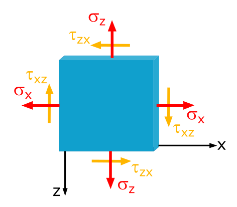
Sheet with given stresses.
Fig. B1.3: Sheet with Given Stresses

Determine the magnitude and direction of the principal stresses.

Solution

For the given \(x\), \(z\)-coordinate system, describing a plane where the x-axis points positively to the right and the z-axis points positively downward, and the given stresses \(\sigma_x\), \(\sigma_z\), and \(\tau_{xz}\), we can use the formula 1.10xz to determine the principal stresses:

Continue with TechMechAcademy+

Everything. Always. Everywhere.

With TechMechAcademy+ full access to all content.

alt
alt
alt
alt
alt

Are you already a TechMechAcademy+ premium member? Then please log in here to enjoy full access to all content.

Table of Contents
FAQ: How to Open a Link in a New Tab?

There are 3 Ways to open a link in a new tab:

  1. Method 1: Ctrl+Click

    The first method requires a keyboard and a mouse or trackpad. Simply press and hold the Ctrl key (Cmd on a Mac) and then click the link in your browser. The link will open in a new tab in the background.

    Note: If a link points to content on the same page, it is not possible to display that content in a new tab using this method.

  2. Method 2: Mouse Scroll Wheel

    If you use a mouse with a scroll wheel, you have one of the easiest ways to open links in new tabs. Simply put the cursor over the link and click the scroll wheel. The link will open in a new tab in the background.

  3. Method 3: Right-Click Menu

    The last method is probably the one most people know. but it's not as quick as the other methods. When you see a link you want to open in a new tab, right-click it. You can then select "Open Link in New Tab" from the menu.