Max Value | TechMechAcademy

Step 4: Deriving the Formulas for Normal Stress $\sigma_\xi$ and Shear Stress $\tau_{\xi\eta}$ from Previous Results

Mohr's Circle for Uniaxial Stress State - The Equation

On this Page

Practice Exercises

Table of Contents

For which Angles $\varphi$ are the Normal Stress $\sigma_\xi$ and the Shear Stress $\tau_{\xi\eta}$ Maximum?

Hey, this is a really exciting topic, isn't it?

Now we're going to find out when the normal stress and shear stress in a uniaxial stress state are at their greatest. So, buckle up, it's going to be exciting!

Let's imagine we have a bar:

It is stretched or compressed at one end..
There are then stresses inside the bar.
We can decompose these stresses into normal stresses and shear stresses.

Okay, but when are these stresses at their greatest?

To understand the solution, let's first dig up the formulas for normal stresses and shear stresses developed in the previous steps:

Normal stress for rotated coordinate systems/arbitrary cutting angles:

$$ \begin{aligned} \sigma_\xi = \dfrac{\sigma_x}{2}\bigl(1+\cos(2\varphi)\bigr) \end{aligned} $$

(1.4)

Shear stress for rotated coordinate systems/arbitrary cutting angles:

$x$,$y$-system

$$ \begin{aligned} \tau_{\xi\eta} = -\dfrac{\sigma_x}{2}\bigl(\sin(2\varphi)\bigr) \end{aligned} $$

(1.5_xy)
$x$,$z$-sstem

$$ \begin{aligned} \tau_{\xi\eta} = \dfrac{\sigma_x}{2}\bigl(\sin(2\varphi)\bigr) \end{aligned} $$

(1.5_xz)

Interesting: The cutting angles $\varphi$ at which the normal and shear stress are each maximum occur in the sine and cosine functions.

Let's take a closer look at these two functions:

This figure shows the sine and cosine functions in the range of -Pi/2 to 2Pi. — Fig. 1.2.12: Sine and cosine function

For our cutting angle $\varphi$, only a small section of the image is actually interesting: the one between $\varphi=0$ (perpendicular cut) and $\varphi=90°$, which corresponds to $\varphi=\frac{\pi}{2}$ (in radians).

Aha! There's something great to discover here!

The sine curve reaches its minimum value of 0 at $\varphi=0$ and its maximum value of 1 at $\varphi=\frac{\pi}{2}$.
The cosine curve reaches its minimum value of 0 at $\varphi=\frac{\pi}{2}$ and its maximum value of 1 at $\varphi=0$.

That's great, but when are the stresses at their greatest?

Let's start with the normal stress:

In Eq.(1.4) we find the cosine - it is maximum when its argument is 0, i.e. for $\varphi=0$.
So the normal stress is greatest when you cut the bar perpendicularly.
This is exactly perpendicular to the axis of the bar.
In this case, the shear stress is zero.
Can you imagine that? It's like the "strongest" cut.

And the shear stress?

In Eqs. (1.5_xy) and (1.5_xz) we find the sine - it is maximum when its argument is $\frac{\pi}{2}$.
Watch out, it's a trap! Since the angle $\varphi$ does not appear alone as the argument, but with the factor 2, in this case it is not $\varphi=\frac{\pi}{2}$, but $\varphi=\frac{\pi}{4}$!
So the shear stress is greatest when you cut the bar at an angle of 45 degrees to the axis of the bar.
Remember: 45 degrees is the magic number!
In this case, the normal stress is half as large as the maximum normal stress.

Here is the formal proof, if needed:

$$ \begin{align} \tag{1} \lvert \sigma_{\xi(max)} \rvert &= \lvert \sigma_{\xi(\varphi=0°)} \rvert = \dfrac{\lvert \sigma_x \rvert}{2}\bigl(1+\cos(2 \cdot 0°)\bigr) = \dfrac{\lvert \sigma_x \rvert}{2}\bigl(1+1\bigr) = \dfrac{\lvert \sigma_x \rvert}{2} \cdot 2 = \underline{\underline{\lvert \sigma_x \rvert}} \\[10pt] \tag{2} \lvert \tau_{\xi\eta(max)} \rvert &= \lvert \tau_{\xi\eta(\varphi=45°)} \rvert =\dfrac{\lvert \sigma_x \rvert}{2}\bigl(\sin(2 \cdot 45°)\bigr) =\dfrac{\lvert \sigma_x \rvert}{2}\cdot \bigl(1\bigr) = \underline{\underline{\dfrac{\lvert \sigma_x \rvert}{2}}} \end{align} $$

Everything clear?

Here are the key points again:

Maximum normal stress
- Perpendicular cut to the rod axis
- Shear stress is zero
Maximum shear stress
- Cutting angle of 45 degrees to the rod axis
- Normal stress is half as large as maximum normal stress

In the uniaxial stress state, the magnitude of the maximum normal stress $\lvert \sigma_{max} \rvert = \lvert \sigma_{x} \rvert$ occurs in the perpendicular section, and the magnitude of the maximum shear stress $\lvert \tau_{max} \rvert = \lvert \frac{\sigma_{x}}{2} \rvert$ occurs in the 45° section $\bigl(\frac{\pi}{4}\bigr)$ to the applied load.

Practice Exercise

Practice Exercise F-1.1.4

The illustration shows a beam with a square cross-section, fixed on the left side. In the drawing, three sectional planes a, b, and c are indicated. Sectional plane a is perpendicular to the beam axis. Sectional plane b runs from the upper left to the lower right, with the given angle Beta describing the smaller angle at the top. Sectional plane c runs from the lower left to the upper right, with the given angle Gamma describing the smaller angle at the bottom. The side length of the cross-section is denoted as d. A tensile force F acts at the right end of the beam at the center of the cross-section.

Normal and Shear Stress at an Arbitrary Section Angle

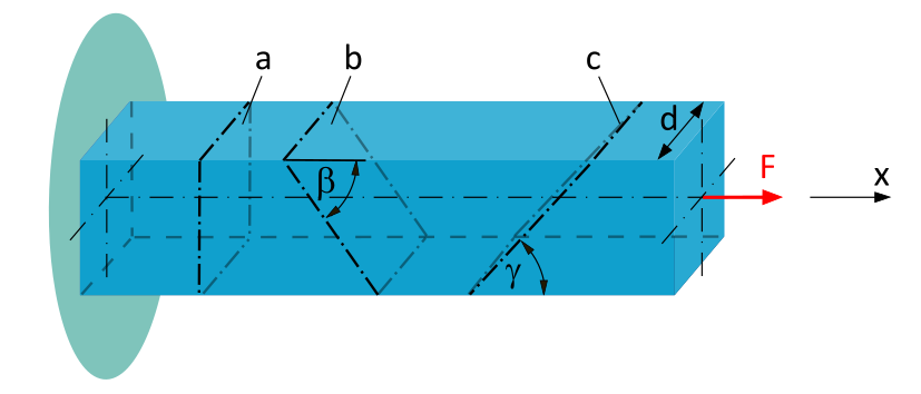
A clamped beam with a square cross-section (side length $d=20~\mathrm{mm}$) is subjected to a tensile force $F=10~\mathrm{kN}$ along the beam axis.

Determine the average normal stress and the average shear stress...

...acting in cross-sectional plane a.
...acting in cross-sectional plane b ($\beta = 50°$).
...acting in cross-sectional plane c ($\gamma = 40°$).

Mechanics of Materials

Stress State: Dive into the World of Forces and Stresses!

For which Angles \(\varphi\) are the Normal Stress \(\sigma_\xi\) and the Shear Stress \(\tau_{\xi\eta}\) Maximum?

Normal and Shear Stress at an Arbitrary Section Angle